Last week we talked about compression, where we went over the basics of compression and the two major categories (lossy and lossless). This week we will be going over a specific example of lossless compression Huffman Coding which is a text compression algorithm that is the predecessor for most current and more complex text compression methods. Before we get into how Huffman coding works, we need to go over some basics of how data is structured in a computer. As most of you know all data in a standard computer is stored in 1s and 0s or bits, every possible file is eventually boiled down to a chunk of 1s and 0s on a disk. We use different sized groups to represent different data types but a for a single English character in a text file we use 8 bits or 1 byte.

So, with that being said text file with each letter being 8 bits the amount of space can add up quickly, not really an issue for modern computers with terabytes of memory but for David Huffman in 1952 it was paramount to find a reliable and lossless compression solution, hence he developed what is now known as Huffman coding (2). Huffman coding takes advantage of statistical redundancies to compress a text file on average 30% which can make a huge difference, and the more statistical redundancies the higher the compression ratio goes up (1).

So, lets get into how Huffman coding works; say we took the title of this Dr. Seuss’ book

“One Fish Two Fish Red Fish Blue Fish”.

Right now, with spaces we have 36 characters in this quote which adds up to a total of 288 bits. Let us see if we can use Huffman code to get that down a little bit, first we need to count the occurrence of each letter (including spaces). Here are the occurrences of the letters in this sentence ordered most to least.

[space = 7, S = 4, F = 4, H = 4, I = 4, E = 3, O = 2, D = 1, W = 1, L = 1, N = 1, B = 1, R = 1, T = 1, U = 1]

As one might expect space is by far the most used character, now we must take this data and build it into a tree. Here is a quick video to show you how the tree is built.

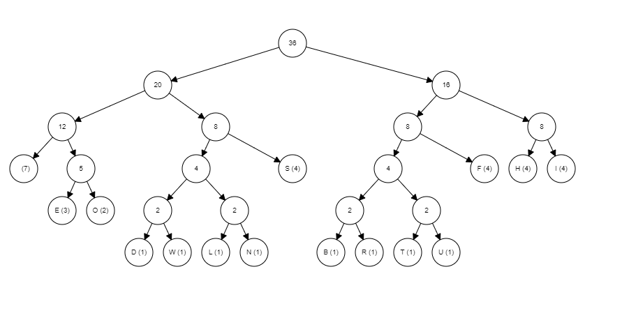
As you can see these graphs can get large pretty quick hence why I chose a sentence with a limited number of letters, now to interpret the graph. To interpret the graph, you need to know that any traversal to the left represents a zero and any traversal to the right represents a 1 and you always start from the root (node with the number 36 in it in this example). For example, the letter ‘S’s traversal from the root is left -> right -> right which is equal to 011 so now S can be represented as 011 five whole bits less than it was being presented by. Here is a list of the rest of the letters and their new bit representation.

[space = 000, S = 011, F = 101, H = 110, I = 111, E = 0010, O = 0011, D = 01000, W = 01001, L = 01010, N = 01011, B = 10000, R = 10001, T = 10010, U = 10011]

Now all letters are below 8 bits, therefore making the file compressed now adding up all the new bit amount times the frequencies of that letter the new total amount of bits used is 129 much less than the original 288, a whopping  55.2% reduction in size. Side note here Huffman Coding will not always make letter or symbols below 8 bits, when the tree gets large enough letters with very low frequency will go beyond 8 bits but this is still outweighed by the drastic reduction in bits used to represent the more used letters. Overall, compression is a very deep an interesting subject with a lot of detailed and interesting different methods for reducing file size; I encourage to look up other forms of compression for yourself.

Sources:

                1. https://www.youtube.com/watch?v=JsTptu56GM8&t=1s

                2. https://en.wikipedia.org/wiki/Huffman_coding

Compression while less as important than it used to be with storage becoming cheaper and bandwidth getting larger; compression is still a vital way to transfer files faster and free up storage. For large data warehouses maintained by big companies like google and amazon reducing the data you store and transfer by any amount will reduce the amount of computing power needed and the storage need; therefore, resulting savings (1).  Compression in short is the reduction of space a file uses to store the same information or in some cases approximately the same information. All forms of compression in computer science use some form of encoding and decoding. Meaning that to compress a file or transmission you encode it using a certain algorithm or process to convert the data into a specific format that will still have the ability to be decoded approximately into the original data. Compressing a data file like whenever you zip a file is usually called data compression, but when data is compressed to be transferred it is call source coding.  For both types the devices or processes that compress the data are referred to as the encoder and the devices that uncompress are called the decoder (2). The major trade off of compression is the time complexity; if you are compressing a video to transmit to the user the amount of time it takes to decode could result in a poor user experience. Overall there are many different forms and algorithms for compression that deal with the space time complexity trade off, most with logically designed for certain uses, and we will talk about a particular forms of compression in later blog posts but for now we will talk about the two major categories of compression known as lossy and lossless (2). We will first talk about the more straight forward of the two lossless compression.

Lossless

Lossless compression simply put is just compression that from encoding to decoding does not lose any data. Meaning that if you encode a file than decode a file you get the exact same file with the size and values being exactly the same. This is usually done by taking advantage statistical redundancies in data, for example if you were to compress this blog post you might have far more ‘e’s and ‘i’s than ‘q’s and ‘z’s, or if you have a digital photo of “The Starry Night” you would have a lot more blue green pixels than red and purple. As of now each pixel and letter is represented by the same amount of binary memory but since we have a lot more of a certain type of data, we can encode it so that the more used type of data is now represented by a smaller amount of binary memory (2). This is a more data specific form of compression but allows us to not lose any of the original contents of the data before it was encoded.

Lossy

Whether you know it or not you are probably very familiar with lossy compression. If you’ve ever seen an image that looks extremely blurry on the internet that not necessarily because that image was taken on the first camera phone ever but because it has been shared so many times between websites and people; going through lossy compression over and over again that it has lost a lot of its detail. If you haven’t been able to gather lossy compress is the opposite of lossless where some of the original information is lost when it is compressed (2). Forms of lossy compression are much more complicated and actually usually rely on the psychology, and how the data is perceived using thing like what will be the focal point of an image or what variants of color can the human eye perceive well, or what wavelength of sound can the human ear hear as there is no point in spending extra to stream music so your dog can enjoy it too . In short lossy compression decides what data is important and what data is not important then encodes accordingly.

I hope this blog was interesting to you and gave you a high-level explanation on how compression works in computer science.

Sources:

https://csfieldguide.org.nz/en/chapters/coding-compression/

https://en.wikipedia.org/wiki/Data_compression

Today we are going to talk about a fundamental concept in programming, loops, and iterators. Loops and iterators are some the most common programming concepts and you will find them in one form or another in almost all modern programming languages. Lets first start with loops; loops are used when you have a repeating routine or sub routine, where you may be calling a whole function multiple times, or just executing a simple piece of code the important part of loops is that is an easy and modular way to execute a  sequence of code multiple times.             For these examples we will be using ruby as is very readable and has a lot of different loops and iterators, but we will not touch on all of them. First and most simple loop is while loops; while loops will execute the piece of code while a condition is met hence while loop. Real life example would be while meat is raw cook; here is a code example of a while loop in ruby.

x = 5
while x <= 0
  puts x
  x = x - 1
end

This simple piece of code will just run and minus one from x until it is zero, nothing fancy put hopefully its helpful. Here is another diagram.

For our next loop we will cover for loops another extremely common type of loop. For loops like while loops it executes the loop while a condition is met but it only revolves around an increasing value, with that value being automatically updated right when the condition is called. Here is an example of a for loop.

x = 5
for i in 1..x do
  puts i
end

This section of code will update i until it is equal to x which in this case is 5, and with each pass over of the loop it will print it. So, the console will print 1, 2, 3, 4, 5 (each in a newline without comma). For good measure here also how to do this same code in a while loop, as well as a diagram of how for loops work.

x = 5
i = 1
while i <= x
  puts i
  i = i + 1
end

Now that we’ve cover the two most common loops let move onto iterators. Iterators are an object that allows us programmers to traverse a container of elements/values, most commonly lists (1). For these examples we will be using arrays; the type of iterator we will be using today is “dot each” or written code as .each. Dot each is what it is called in Ruby but it is commonly called For each in other languages with a slightly more complex syntax. Dot each will simply iterate over every element of the list and execute some piece of code for each element. Here is the syntax for a dot each iterator in Ruby.

names = ['Bob', 'Joe', 'Steve', 'Janice', 'Susan', 'Helen']
x = 1

names.each do |name|
  puts "#{x}. #{name}"
  x += 1
end

In this example given the array of names you are printing x which is counting with the names and the name itself.

I hope this brief demonstration of loops and iterators was helpful, please look up more documentation on loops and iterators if you are curious. Make sure to look up all the types of iterators and loops in your language of choice as they might add much readability and efficiency to your project.

Sources:

1. https://en.wikipedia.org/wiki/Iterator#:~:text=In%20computer%20programming%2C%20an%20iterator,provided%20via%20a%20container’s%20interface.
2. https://launchschool.com/books/ruby/read/loops_iterators

I’ve always known a little CSS, but it has never been my strongest skill set, as there are many properties of CSS and the ways they interact is not always clear and can be unexpected. So, this week I decided to further my skills and learn how to do CSS animations using keyframes, which make the process of creating animations surprisingly simple.

Before learning about keyframes we first need to learn about CSS transitions and transformations. There are many transitions you can do in CSS but it is a common held belief that you should only really only transition four things for performance reasons if you are adding your transitions to a big app or working on productions level code you should definitely stick to these four but if you are just making some cool stuff in CSS feel free to look up more.

	transform: translate()
	transform: scale()
	transform: rotate()
	opacity

Transform translate can take in one to two inputs and basically allows you to move the element by a varying amount in any directions. Transform scale simply allows you to shrink or enlarge an element and rotate and opacity are both pretty self-explanatory. So, with these tools along with keyframes we can make some pretty cool CSS animations.

Keyframes follow a pretty simple syntax but requires some values first:

  	animation-name: name;
  	animation-duration: 10s;
  	animation-timing-function: linear;
  	animation-delay: 0s;
  	animation-iteration-count: infinite;

The animation-timing-function is how fast you want certain parts of the animation to move at certain times, here its linear it will move at the same continuous speed. So, if you were animating a car it would move across uniformly, but if you want to make it look like the car was speeding up maybe you’d use an exponential timing function. The rest of the animation properties are pretty straight forward, so I won’t go over them. Then the actual syntax of the keyframe:

@keyframes name {
  0% {
  }
  25% {
  } 
  50% {
  }
  75% {
  }
  100% {
  }
}

Each one of these percentage fields are where you put your transformation and other values, where each percentage value is the percentage through the animation. Important to note you are not limited to four values only at these four percentage values but can have anywhere between one and 100 values (each value could be 1% {}, 2% {}, …, 100% {}). Within each of these percentage values you write your transformation for example if you wanted the HTML element to grow in size and change colors you’d have something like this.

@keyframes changeColorsMakeBig {
  0% {
    transform: scale(2);
    background: red;
  }
  25% {
    transform:  scale(1);
    background: green;
  } 
  50% {
    transform:  scale(2);
    background: pink;
  }
  75% {
    transform:  scale(1);
    background: orange;
  }
  100% {
    transform:  scale(2);
    background: yellow;
  }
} 

So, this animation would change the elements colors and oscillate the size back and forth. So now you have the basic tools to make animations, there are many fun and cool examples of animations made with key frames you can find all over the internet, but codepen is a good place to start and codepen also makes it easy to test out your own animations.

I am by no means an expert on databases but if you are starting a project, there is always questions to ask about said project that can be answered in making user stories, flow-charts, objectives, constraints and so, but one of the most important parts of any application is how you store data. That’s where based one the purpose and nature of your application will determine whether to use a relational or non-relational database, and I hope to define what it is, and what the advantages and disadvantages of each are and when they should be used.

Relational Database

            A relational database if you could have guessed is a database based on the relational model of data. Where each database is a collection of tables each with defined and finite data where that data is related to one another. Each table columns where it can have multiple data types, for example if you were storing customer information, you’d have a customer table like this with your columns organized First name, Age, Date of birth, all three can be different datatypes. Relational databases most commonly use a structured query language or commonly called SQL to access the tables this is a high-level language where you nest statements and in almost plain English tell the database what to give you in return. Some examples of common relational databases are MySQL, PostgreSQL, and SQLite.

Non-relational Database

            Non-relational again if you could have guessed are just databases that do not relate. Data is not structured in rows and columns but are more stored as a collection, more specifically usually in some form of JavaScript Object Notation or more commonly known as JSON but they can usually import formats. The language non-relations databases use again predictably is called NoSQL which acts the same as SQL in the sense that it is used to write and read to databases but works to find key value pairs rather than finding specific table and values. Non-relational databases have dynamic schema meaning they do not have predetermined schema so a value (“column”) can be added whenever you want, where for relational you can only add new inputs to a table (rows). This makes relational databases vertically scalable and non-relational horizontally scalable. Examples of non-relational databases are MongoDB, CouchDB, and Redis.

Advantages and Disadvantages of Both           

Overall after learning what both database types are its pretty clear to see where one would be a much better than the other. Relational databases are great for having a predetermined schema, and data that relates to each other. But keeping these relations up to date and making sure they can match up can be difficult for some applications at full scale especially for huge application with data stored in many different locations. Usually larger amount of data you must store in different tables the more likely you should be using a non-relational database but if your database is relatively few tables and relies a lot on how the data is connected the relational database is a great choice. As a relational database adds a lot of functionality a non-relational can’t with having automatic joins and verifications, where a lot of these action must be manually done on a non-relational database. In conclusion there is both advantages and disadvantages to both but it’s about finding the right balance to figure out which database is best for your applications.

Sources:

1. https://www.pluralsight.com/blog/software-development/relational-non-relational-databases#:~:text=Relational%20databases%20like%20MySQL%2C%20PostgreSQL,in%20collections%20of%20JSON%20documents.
2. https://en.wikipedia.org/wiki/Relational_model

Recursion in short can be described as a divide and conquer method of solving a problem in computer science. With the first step being to divide a problem into smaller subproblems then dividing those subproblems and so on. Until the problem cannot practically be divided down any more then solve the smallest subproblem then use that solution to go back up a level and solve the next smallest sub problem and so on until you arrive at the original solution. If graphed this process could be represent as a tree, with the trunk being the original problem and the branches being the subproblems and the leaves being their subproblems.

If you haven’t realized it probably the most difficult part about recursion is describing it while in practice it can be mind-bending at times overall it is pretty simple to implement. In fact, the idea of recursion is by no means exclusive to computer science nor a recently developed process being used back in 1888 by Dedekind to as notation to describe natural numbers (2). Recursion in general is more of a concept used in computer science classes and in older languages that don’t have built in for loops like scheme languages. It is a slightly slower method than many iterative methods of problem solving, and has some risk of stack overflow but can be used in production code if it is easier to conceptualize and therefor makes for quicker to develop, it is commonly used in tree or graph searches (3).

There are two key concepts every recursive function has the base case and the recursive case.

1. The base case: where the function checks if it’s in the smallest subproblem and then will return the solution. This must be checked for before the recursive case.
2. The recursive case: the case in which the function divides the problem, then inputs the subproblem into a function call of itself.

A simple example of a solution using recursion is solving a factorial.

function factorial(n) {
  // Base case
  if (n === 0 || n === 1) {
    return 1;
  }
  // Recursive case
  return n * factorial(n — 1);
}

For this example if you called factorial(3), the order of returns would look like this:

1. factorial(3) will return 3 * factorial(2)
2. factorial(2) will return 2 * factorial(1)
3. factorial(1) will return 1 (as n now equals 1)

So if we substitute:

1. factorial(3) returns 3(2*factorial(1))
2. factorial(3) returns (3(2(1))) = 6 (or 3! )

So the first call to return is factorial(1) which causes a chain reaction for all the other call to return till the final solution (5).

So, when designing a recursive function, the most important part is to first figure out the base case, which is usually just simple check then a return of a static value or the input value. For example, if doing tree traversal your base case checks if the node is null then just returns nothing if it is. Then find the recursive case which can be a little trickier but is usually just making one or two call to the same function with the input being some a modified version of the original input. In general recursion can seem confusing and daunting when first learning it as is something that is difficult to understand on paper but once you start writing some recursive programs it will seem much easier.

Check out this simple recursive Sudoku solver I wrote in java.

https://github.com/EricStukenberg/SudokuSolver

Sources:

1. https://ericstukenberginfo.data.blog/wp-content/uploads/2020/06/7bd81-1w2ljumwtkjgldz01qsqiyg.gif
2. https://en.wikipedia.org/wiki/Recursion_(computer_science)
3. http://www.people.cs.uchicago.edu/~soare/History/compute.pdf
4. https://arstechnica.com/civis/viewtopic.php?f=20&t=1142971#:~:text=Recursion%20is%20(in%20many%2C%20but,valuable%20tool%20for%20production%20code.
5. https://medium.com/@daniel.oliver.king/getting-started-with-recursion-f89f57c5b60e

The reality is that no matter how good you are at programming you will almost never get complex code to run correctly the first time. In turn, having good debugging practices is one the most valuable skills a programmer can possess. Debugging has been described as “being a detective in a crime movie where you are also the murderer”, which almost makes debugging sound like it would be an easy case to solve. So, I’d like to add to that and say that debugging is like being a detective in a crime movie where you are also the murderer, you have no recollection of committing the crime, and your only clue is an obscure anonymous message that keeps appearing, and sometimes slightly changing while never getting more helpful. As all programmers know trying to resolve bugs can be some of the most mundane and frustrating parts of software development and can lead to many, many, hours of squandered time that you’d rather spend building out new functionality, but it is part of the reality of being a programmer.

First, let’s go over the few general but important steps of debugging.

1. Try to avoid writing bugs in the first place. This may seem obvious but writing sloppy and confusing code will almost always lead to more and harder to solve bugs. Making sure that your code is very readable, modular and well documented will go much further in creating bug free code than any of the following steps will.

2. Run your code more often after small changes. Similar to step one this is more of a step to avoid creating bugs but also catching a bug early before they stack on top of each other and become harder to find. If you are trying to build out a functionality, make sure to test each tiny sub problem that will eventually all come together to create the functionality.

3. Understand the error/bug. One of the most effective ways to squash a bug is to fully understand what the error is and exactly what is causing it. This is always the first step in actually resolving it. You must first be able to recreate the bug consistently to get the gist of where and how in your code the bug is being created. Secondly use your resources around you, google the error message, read forums of what others have run into as to why the bug is there, ask colleagues. You never know where the answer will come from but once you know where and why that bug is there that is 90% of the battle of resolving it.

4. Use debugging tools. Although this is kind of the same as Step 3 to use your resources, it can be hard to even know what questions to ask or what to google when you are completely in the dark as to what is happening. Using automated tests and debugging tools can give you key knowledge and is much more insightful and meaningful than is putting a bunch of print statements or console logs everywhere.

For instance if you want to use Chrome debugger for vs code when you’re writing web applications, heres a quick setup tutorial. First thing that you’re going to want to do is download the for chrome extension on VS code. After which for your particular project you are going to want to add the debugging features via a launch.json file. To do so click on the debugging icon located on the left toolbar. Then change the url from “http://localhost:8080” to “http://localhost:3000/” or whichever port your app is running on, then save the file. This will now attach the VS debugging tools to the instance of chrome that you will open your project in.

In conclusion, having debugging skills is an extremely important part of a part of a programmer’s arsenal. Having and honing these skills will save you valuable time and insure more efficient and affective code.

Fetch is the most convenient way for JavaScript developers to make any kind of HTTP request to a server. Fetch will gather or upload data asynchronously meaning that although JavaScript is a single threaded language (one process at a time) fetch can do its work in the background while it waits for the server to respond in order to not stall and bottleneck your code. This is done using ES6 Promises which take advantage of the micro-task queue which is a higher priority queue which will return before the callbacks inside the message queue, so it can return and be executed before the currently running process in a way (1). Here is useful diagram of an asynchronous process in JavaScript.

Fetch has a total of five main methods GET, POST, PATCH, PUT, DELETE, and HEAD, I will be covering five of them (GET, POST, PUT, PATCH, and DELETE). Fetch actually only returns a promise so we must use a special function called “then” that waits for a promise to get fulfilled and then the “then” function can be used to return the data or to be used in a different ways. First and most simple is the GET method which is formatted like this.

As you can see this function simply makes a request to a URL then once that promise is fulfilled returns the data in JSON form then console logs that data. Then the catch is always a good idea to handle errors so you know what error you ran into. The Second method I will talk about is POST, this is when you a create new data to send and be saved to the database or file. This follows the format of first declaring the fetch and the URL then inside the fetch you must specify the method type (POST), headers, and body. So for example if you had a database full of users you could create a user like so.

The content type in the header specifies what the media type is that is being sent to the server, in this case JSON. Next the body is just the data itself that is being sent in this case we formate it with JSON.stringify to properly input it into the database. The next method is PUT which is similar to POST method but is used to update an existing resource rather than creating a new one, here is an example of a PUT.

As you can see PUT is very similar to POST but the URL it goes to is slightly changed to be the exact content in the database you are trying to change. An even more similar fetch method is PATCH, which is exactly the same as PUT but with two exceptions method: ‘PATCH’ obviously, and the data being passed in does not need to be a whole user object (or whatever table in your db you’re trying to change). It can just be the key value pairs of the objects fields you are trying to change. Example

body: JSON.stringify({username: Jason})

This will go to the indicated URL and only update the username and does not need to pass in a full user object like PUT.

Lastly the simplest method DELETE doesn’t need all of the headers or anything it just needs the exact path of the DB resource and the method DELETE.

Thats all the basic information you need to start using fetch in your projects I hope it was helpful.

Sources:

1. https://blog.bitsrc.io/understanding-asynchronous-javascript-the-event-loop-74cd408419ff

Images:

1. https://www.sencha.com/wp-content/uploads/2016/03/asynch-javascript-promises-img2.png

Software development as most of us know is a very fast-moving industry. New frameworks and languages are being developed all the time. Today I’d like to talk about a relatively new programming language Kotlin. Released in 2016, Kotlin had been in development since 2010 by JetBrains. Kotlin is a general-purpose programming language that is closely related to Java, even going as far as naming the language after an island just like Java was when it was created all the way back in 1995. Kotlin is designed to work in conjunction with the Java Virtual Machine (1). The Java Virtual Machine (JVM) is simply a virtual machine that allows any machine to run Java or Kotlin or any other JVM language by creating the framework of compiling your code into Java bytecode, a low-level code related to machine code, and then to machine code to be run on your machine.

Plainly put, Kotlin was designed to directly replace Java by being a better programming language but still retaining all the power and versatility of Java. The strong link with Java is cited as being another strength as it allows companies to make a gradual seamless transition from Java to Kotlin (2). Kotlin’s biggest advantage over Java is its conciseness. Kotlin can declare classes, declare data structures and solve many complex problems in one tenth the amount of code as Java. This allows programmers to code faster without being bogged down in the time-consuming realm of syntax. It also enables the creation of code with a much higher level of readability and inherently makes coding safer as it prevents programmers from making mistakes that are common in less powerful languages (3). Overall, conciseness and readability can be a huge advantage for individual programmers and companies alike. Another big advantage is that it allows coders who are new to the language to learn it much quicker than most other languages and allows experienced programmers to code much faster and efficiently giving an additional productivity boost to companies. In fact, for this very reason since the introduction of Kotlin into Android studio Kotlin has surpassed Java as the preferred language of Android app developers (1). Here is an example of Kotlin class creation vs Java.

As a software developer it is always exciting to learn about new technologies and languages. In my opinion always having the necessity to continue learning is one of the best parts of being a programmer. While I don’t think Java is going anywhere, Kotlin’s ease of use and the lack of 25 years of bundled legacy code, makes Kotlin an extremely appealing option for any savvy programmer. Overall, Kotlin is more of an iteration of Java, a step forward for an aging language, which is making a best effort to boil down the core principles and make a better language out of it.

If curious here is a long list of direct differences between Java and Kotlin from a great blog written by Vijay Singh (link to blog: https://hackr.io/blog/kotlin-vs-java)

Java vs Kotlin: Comparison

Sources:

1. https://kotlinlang.org/api/latest/jvm/stdlib/index.html
2. https://www.jrebel.com/blog/interview-with-kotlin-creator-andrey-breslav
3. https://business.udemy.com/blog/kotlin-vs-java-9-benefits-of-kotlin-for-your-business/
4. Vijay Singh’s blog post: https://hackr.io/blog/kotlin-vs-java

Image 1: https://image.slidesharecdn.com/ivankrylov-lifecycleofajitcompiledcode-180530151711/95/lifecycle-of-a-jit-compiled-code-4-638.jpg?cb=1527693632

Image 2: https://www.mediaan.com/wp-content/uploads/2019/02/Java_vs_Kotlin.png

               Today I would like to talk about my personal favorite sorting algorithm, radix sort. I realize that even saying I have a favorite sorting algorithm I just outed myself as a complete utter nerd although in my view that ship sailed a long time ago. In short radix is a sorting algorithm that uses the digits of each individual element in an array to put the elements into corresponding ‘buckets’ and then orders the array in the corresponding order of the buckets. The algorithm then proceeds to go over the new array again and again until the elements are all sorted. Here is a gif to make that a little less confusing.

Radix sort is actually one of the oldest sorting algorithms developed. It was developed all the way back in 1887 by Herman Hollerith which means that radix sort was developed before even the invention of the ballpoint pen let alone a modern computer (Herman). The algorithm was originally created for use in the tabulating machine that developed for the 1890 US Census to summarize punch card information (Columbia). Radix sort did not come back into use again until the 1920’s when it was found to be an efficient way to sort punch cards and was used by companies like IBM.

Radix sort was eventually computerized in 1954 by the MIT professor Harold H. Seward bringing it into the modern era. Now radix can be used for a variety of collections but most commonly integer or binary string collections. Compared to some of the ‘newer’ sorts, radix sort may seem to lack some complexity but that is its charm. In my opinion radix sort shows the ingenuity of Herman Hollerith invention at a time when there were not organized concepts of programming languages or programmable computers.

Radix sort is neither the quickest nor the slowest sorting algorithm, coming somewhere in the middle in terms of time required to complete a sort. Where radix earns respect is it is one of the most consistent, where worst and best case are both O(nk). Along with this, it is a non-comparative algorithm meaning that no two objects in the collection are ever compared to each other. For me personally I love radix sort as it was the first sorting algorithm that I learned about where it seemed to be a genuinely unique solution. Its uniqueness made me think differently about sorting and computer science in general. Whenever I program and have to sort something, make a visited hash, or any kind of key value pair I think back to radix sort as it was the first aha moment of my programming career, and it reminds me how truly great coding is when you can have such limitless solutions for a single problem.

RUBY CODE:

  def radix_sort(base=10)
    ary = dup
    rounds = (Math.log(ary.minmax.map(&:abs).max)/Math.log(base)).floor + 1
    rounds.times do |i|
      buckets = Array.new(2*base){[]}
      base_i = base**i
      ary.each do |n|
        digit = (n/base_i) % base
        digit += base if 0<=n
        buckets[digit] << n
      end
      ary = buckets.flatten
      p [i, ary] if $DEBUG
    end
    ary
  end
  def radix_sort!(base=10)
    replace radix_sort(base)
  end

Sources:

HERMAN, HOLLERITH. ART OF COMPILING STATISTICS. US395781A, 1889.

Cruz, Frank. “Columbia Difference Tabulator.” Columbia Difference Tabulator, http://www.columbia.edu/cu/computinghistory/packard.html.

Code: https://rosettacode.org/wiki/Sorting_algorithms/Radix_sort#Ruby